When you begin to research a field of study, you often get overwhelmed by the amount of existing knowledge you have to learn before you could go further. One useful way to bootstrap yourself is to only learn a minimal amount of basic ideas that are enough for you to “survive” in the field. Such basic ideas are the Minimal Actionable Knowledge & Experience (MAKE) of the field. Here, I will try to present the “MAKE” of the field of fast matrix computations.

Low-rank matrices and important information

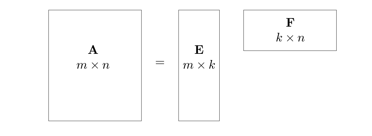
An $m\times n$ matrix $\mathbf{A}$ is low-rank if its rank, $k\equiv\mathrm{rank}\,\mathbf{A}$, is far less than $m$ and $n$. Then $\mathbf{A}$ has a factorization $\mathbf{A} =\mathbf{E}\mathbf{F}$ where $\mathbf{E}$ is a tall-skinny matrix with $k$ columns and $\mathbf{F}$ a short-fat matrix with $k$ rows.

For example the following $3\times3$ matrix is of rank-$1$ only.

$$\begin{bmatrix} 1 & 2 & 3\\ 1 & 2 & 3\\ 1 & 2 & 3 \end{bmatrix} = \begin{bmatrix} 1\\ 1\\ 1 \end{bmatrix} \begin{bmatrix} 1 & 2 & 3 \end{bmatrix}$$

Given a matrix $\mathbf{A}$, there are many ways to find $\mathrm{rank}\,\mathbf{A}$. One way is to find the SVD

$$\mathbf{A}=\mathbf{U}\mathbf{\Sigma} \mathbf{V}^*$$

where $\mathbf{\Sigma}=\mathrm{diag}(\sigma_1,\sigma_2,\dots)$ is an $m\times n$ diagonal matrix, whose diagonal elements are called the singular values of $\mathbf{A}$. Then $\mathrm{rank}\,\mathbf{A}$ is the number of nonzero singular values.

The SVD tells you the most important information about a matrix: the Eckart-Young theorem says that the best rank-$k$ approximation of $\mathbf{A}=\mathbf{U}\mathbf{\Sigma} \mathbf{V}^*$ can be obtained by only keeping the first $k$ singular values and zeroing out the rest in $\mathbf{\Sigma}$. When the singular values decay quickly, such a low-rank approximation can be very accurate. This is particularly important in practice when we want to solve problems efficiently by ignoring the unimportant information.

An interesting example is the $n\times n$ Hilbert matrix $\mathbf{H}_n$, whose $(i,j)$ entry is defined to be $\frac{1}{i+j-1}$. $\mathbf{H}_n$ is full-rank for any size $n$, but it is numerically low-rank, meaning that its singular values decay rapidly such that given any small threshold $\epsilon$, only a few singular values are above $\epsilon$. For example with $\epsilon=10^{-15}$, the $1000\times1000$ has numerical rank $28$.

Other examples of (numerically) low-rank matrices include the Vandermonde, Cauchy, Hankel, and Toeplitz matrices, as well as matrices constructed from smooth data or smooth functions.

As it turns out, a lot of the matrices we encounter in practice are numerically low-rank. So finding low-rank approximation (e.g. in the form of $\mathbf{A}=\mathbf{EF}$ at the beginning) is one of the most important and fundamental subjects in applied math nowadays.

Data sparsity and rank structured matrices

Matrix sizes have been growing with technological advancements. Many common matrix algorithms scale cubically with the matrix size, meaning that even if your computing power grows 1000 times, you could only afford to solve problems that are 10 times bigger than before. These common algorithms include matrix multiplication, matrix inversion, and matrix factorizations (e.g. LU, QR, SVD). Therefore, it is important to speed up these matrix computation methods in order to fully exploit the ever growing computing power.

One major strategy to accelerate the computations is to exploit the data sparsity of a matrix. Data sparsity is a deliberately vague concept which broadly refers to the kind of internal structures in a matrix that can help make computations faster. Following are some common examples of data-sparse matrices.

• The most classcial data-sparse matrices are the sparse matrices, ones with a large number of zero entries. Using compressed data formats, you can save a lot of memories by storing only the nonzero entries (together with their positions). You can greatly reduce computation time by only operating on the nonzero entries while maintaining the sparsity of the matrices (i.e., avoid introducing more nonzero entries). Common sparse matrices include diagonal/block-diagonal matrices, banded matrices, permutations, adjacency matrix of graphs, etc.
• Low-rank matrices, as we have introduced above, are ones admit low-rank factorizations. Commonly used factorizations include the reduced SVDs, interpolative decomposition, CUR decomposition, rank-revealing QR factorizations, etc. Normally the SVD algorithms are more expensive, so the other algorithms are preferred when possible; for very large matrices, all the factorization algorithms can be further accelerated by randomization techniques.
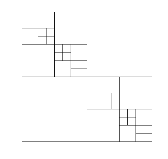
• Rank structured matrices. These matrices are not necessarily low-rank, but can be split into a relatively small number of submatrices, each of which is low-rank. For example, the picture below shows the structure of a Hierarchically Off-diagonal Low Rank (HODLR) matrix, where all the off-diagonal blocks, big or small, have similar ranks. Such structure can for example arise from gravitational or electrostatic interactions, where the diagonal blocks represent the local interactions and the off-diagonal blocks represent the far interactions; the far interactions are low-rank because they are much smoother than the local interactions. Other rank structured matrices include the Hierarchically Semi-separable (HSS) matrices, the inverse of banded matrices, and the more general $\mathcal{H}$-matrices and $\mathcal{H}^2$-matrices. Rank structured matrices can be efficiently handled using tree structures. Matrix algorithms designed for these matrices can be very fast, with computation time scaling linearly or log-linearly with the matrix size.

• Complementary low-rank matrices are a special type of rank structured matrices that can be decomposed by the butterfly factorization (BF). The BF is inspired by ideas of the FFT algorithm (divide-and-conquer and permutations), which can be explained using the butterfly diagram. Butterfly algorithms were initially motivated by solving oscillatory problems such as wave scattering.

With these ideas above, plus a little coding experience with some simple rank structured matrices (a good place to start is with the first two of these tutorial codes), you are equipped with the “MAKE” that gets you ready for going on an advanture to the fast computations with matrices. All the details and other more advanced topics can be learned later once you dig far enough.